In this post we are going to develop the Long Short-Term Memory Recurrent Neural Network LSTM Trading System. We will use this LSTM Trading System for day trading. Did you take a look at our course Wavelet Analysis For Traders? In this course we teach you how you can use wavelet analysis in predicting the trend and use that prediction in making better trading decisions. Wavelet analysis is very popular with hedge fund quants. They use wavelet analysis in making predictions on different instruments.By combining wavelets with neural networks, much superior results have been achieved by different researchers. Quants never show their trading models. So the only way we can built our algorithmic trading models is by reading research papers and trying to implement them in practice.
You should also take a look at our Macroeconomics For Currency Traders Course. Many retail traders have no knowledge of how to apply macroeconomic models to their trading. Macroeconomics is an important subject that is taught in the universities. Central banks are the most important players in the currency market. Central banks have a number of monetary policy tools at their disposal that they use to control the exchange rates. Central banks can increase/decrease interest rates as well as increase/decrease money supply in the market. You need to know how this is done and how it effects the currency market. In this course we teach you the basics of macroeconomics and how the central banks operate. This course will help you a lot in becoming a better informed currency trader. Did you read the post on how to trade the headline news and magazine cover stories? This is an interesting post that explains how you can trade financial magazine cover stories in your trading.
Long Short-Term Memory Neural Network
Long Short-Term Memory Recurrent Neural Network is bit different than the traditional Neural Networks that use neurons a lot in their architecture. Now I personally don’t believe these neurons have any close resemblance to the human neurons. Read the post on how to use autogressive models in your day trading. Now autoregressive models are linear models that in reality fail to capture the inherent nonlinear price behavior. We can use a neural network to model nonlinear relationships. In this regard Long Short Term Memory Recurrent Neural Network has been claimed to perform better than a traditional neural network. We will see how it performs in this post. If you want to learn more about these LSTM Recurrent Neural Networks, you can watch this video lecture.
In the above video lecture you will learn about recurrent neural networks. During the lecture you will also be introduced to Long Short-Term Memory Recurrent Neural Network. LSTM is best suited for sequential data. Our financial time series is also sequential data. You should also learn R. Python and R are two powerful data science and machine learning languages. I have modeled neural networks on R. I have modeled neural networks on Python. Sometime R is better and sometimes Python is better. Time series analysis is much easier in R as compared to Python. Read this post that explains how to convert time series data into an xts R object. Important question for us is to determine how many lags to use in our model. Take a look at the following Autocorrelation and Partial Autocorrelation plots.
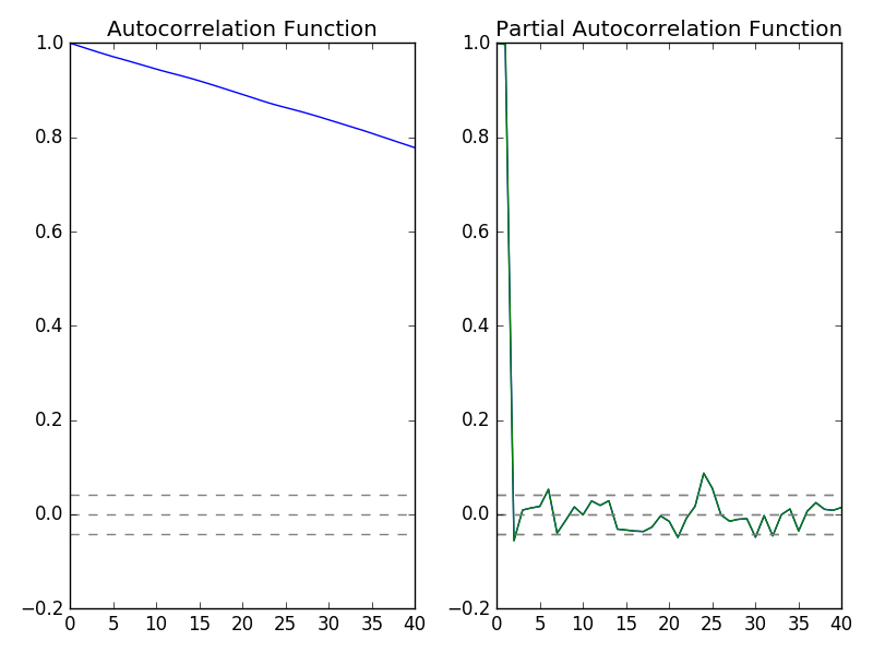
In the above plot, on the left side you can see the Autocorrelation Function plot while on the right you can see the Partial Autocorrelation Function Plot. Autocorrelation function plot shows that data is serially correlated. Now a LSTM Recurrent Neural Network has got an output gate, input gate and a forget gate.Watch the above video in which the professor explains how LSTM network works.
#Long Short Term Memory Recurrent Neural Network For Daily Candle Prediction
import numpy as np
import pandas as pd
import matplotlib.pyplot as plt

#read the data from the csv file
data1 = pd.read_csv('E:/MarketData/GBPUSD1440.csv', header=None)
data1.columns=['Date', 'Time', 'Open', 'High', 'Low', 'Close', 'Volume']
data1.shape
#show data
data1.head()

#explore the data
yt=data1.iloc[0:2286,5]
yt.head()
yt.tail()

#calculate the partical autocorrelations of the time series
from statsmodels.tsa.stattools import acf, pacf
y_acf = acf(yt, nlags=40)
y_pacf = pacf(yt, nlags=40, method='ols')
#plot autocorrelations and particial auto correlations
print(y_pacf)

#Plot ACF:
plt.subplot(121)
plt.plot(y_acf)
plt.axhline(y=0,linestyle='--',color='gray')
plt.axhline(y=-1.96/np.sqrt(len(yt)),linestyle='--',color='gray')
plt.axhline(y=1.96/np.sqrt(len(yt)),linestyle='--',color='gray')
plt.title('Autocorrelation Function')

#Plot PACF:
plt.subplot(122)
plt.plot(y_pacf)
plt.axhline(y=0,linestyle='--',color='gray')
plt.axhline(y=-1.96/np.sqrt(len(yt)),linestyle='--',color='gray')
plt.axhline(y=1.96/np.sqrt(len(yt)),linestyle='--',color='gray')
plt.title('Partial Autocorrelation Function')
plt.tight_layout()

#add time lags to the data
yt_1=yt.shift(1)
yt_2=yt.shift(2)
yt_3=yt.shift(3)
yt_4=yt.shift(4)
yt_5=yt.shift(5)
data2=pd.concat([yt,yt_1,yt_2,yt_3,yt_4,yt_5], axis=1)
data2.columns=['yt','yt_1','yt_2','yt_3','yt_4','yt_5']
data2.tail(6)
data2.head(10)

#drop NaN
data2=data2.dropna()
y=data2['yt']
cols=['yt_1', 'yt_2', 'yt_3', 'yt_4', 'yt_5']
x=data2[cols]
y.tail()
y.head()
x.tail()
x.head()
#transform the data into train and test
from sklearn import preprocessing
scaler_x=preprocessing.MinMaxScaler(feature_range=(-1,1))
x=np.array(x).reshape((len(x),5))
x=scaler_x.fit_transform(x)

scaler_y=preprocessing.MinMaxScaler(feature_range=(-1,1))
y=np.array(y).reshape((len(y),1))
y=scaler_y.fit_transform(y)

#the train set
train_end=2000
x_train=x[0:train_end,]
x_test=x[train_end+1:2286,]
y_train=y[0:train_end]
y_test=y[train_end+1:2286]
x_train=x_train.reshape(x_train.shape+(1,))
x_test=x_test.reshape(x_test.shape+(1,))
x_train.shape


#Long Short Term Memory Network Specifications
from keras.models import Sequential
from keras.layers.core import Dense
from keras.layers.recurrent import LSTM
seed=2017
np.random.seed(seed)
model1=Sequential()
model1.add(LSTM(output_dim=4, activation='tanh',
              inner_activation='hard_sigmoid',
              input_shape=(5,1)))
model1.add(Dense(output_dim=1, activation='linear'))
model1.compile(loss="mean_squared_error", optimizer="rmsprop")

#Time to fit the LSTM model with shuffle set to false we can set it to true
model1.fit(x_train, y_train, batch_size=1, nb_epoch=10, shuffle=False)
model1.summary()
#train and test MSE
score_train=model1.evaluate(x_train, y_train, batch_size=1)
score_test=model1.evaluate(x_test, y_test, batch_size=1)
print( "in train MSE= ", round(score_train, 4))
print ("in test MSE= ", round(score_test,4))

#get the predicted value
pred1=model1.predict(x_test)
pred1=scaler_y.inverse_transform(np.array(pred1).reshape((len(pred1),1)))

#print the predictions
pred1[1:200]

##setup a second LSTM model for Statefulness##
##Model2 calculations take a long time something like 30 minutes##
model2=Sequential()
model2.add(LSTM(output_dim=4, stateful=True, batch_input_shape=(1,5,1),
              activation='tanh', inner_activation='hard_sigmoid'))
model2.add(Dense(output_dim=1, activation='linear'))
model2.compile(loss="mean_squared_error", optimizer="rmsprop")

#Forecaasting One Time Step Ahead
end_point=len(x_train)
start_point=end_point-500
#train the model one epoch at a time with the state reset after each epoch
for i in range(len(x_train[start_point:end_point])):
    print("Fitting example ", i)
    model2.fit(x_train[start_point:end_point], y_train[start_point:end_point],
    nb_epoch=1, batch_size=1, verbose=2, shuffle=False)
    model2.reset_states()
In the above python code we have built 2 models. Model1 is without shuffling and Model2 uses shuffling. Model1 takes hardly a few minutes to complete all the calculations.First we read the input csv file that has GBPUSD Daily data.
Date Time Open High Low Close Volume
0 2008.01.04 00:00 1.9711 1.9849 1.9673 1.9710 17112
1 2008.01.07 00:00 1.9736 1.9756 1.9651 1.9698 16539
2 2008.01.08 00:00 1.9697 1.9827 1.9666 1.9728 18324
3 2008.01.09 00:00 1.9728 1.9762 1.9552 1.9584 18838
4 2008.01.10 00:00 1.9582 1.9662 1.9539 1.9614 19670
Now we separate the closing price using yt variable and then use the shift method to shift this yt into yt_1, yt_2, yt_3, yt_4 and yt_5 as follows:
yt yt_1 yt_2 yt_3 yt_4 yt_5
0 1.9710 NaN NaN NaN NaN NaN
1 1.9698 1.9710 NaN NaN NaN NaN
2 1.9728 1.9698 1.9710 NaN NaN NaN
3 1.9584 1.9728 1.9698 1.9710 NaN NaN
4 1.9614 1.9584 1.9728 1.9698 1.9710 NaN
5 1.9566 1.9614 1.9584 1.9728 1.9698 1.9710
6 1.9559 1.9566 1.9614 1.9584 1.9728 1.9698
7 1.9625 1.9559 1.9566 1.9614 1.9584 1.9728
8 1.9634 1.9625 1.9559 1.9566 1.9614 1.9584
9 1.9714 1.9634 1.9625 1.9559 1.9566 1.9614
We need to remove these NaNs. We do that with the dropna method.
in train MSE= 0.039
in test MSE= 0.1882
Now these are the predictions!
array([[ 1.55317867],
[ 1.55282509],
[ 1.55222237],
…,
[ 1.60890448],
[ 1.6115762 ],
[ 1.61435544]], dtype=float32)
On the other hand, Model2 takes a long time. When you run Model2, it calculates 500 examples as shown below:
Fitting example 486
Epoch 1/1
4s – loss: 6.7802e-04
<keras.callbacks.History object at 0x000001ACB8916FD0>
Fitting example 487
Epoch 1/1
4s – loss: 6.7885e-04
<keras.callbacks.History object at 0x000001ACB889BEB8>
Fitting example 488
Epoch 1/1
3s – loss: 6.7863e-04
<keras.callbacks.History object at 0x000001ACB8909A20>
Fitting example 489
Epoch 1/1
3s – loss: 6.9531e-04
<keras.callbacks.History object at 0x000001ACB892AF60>
Fitting example 490
Epoch 1/1
3s – loss: 6.9805e-04
<keras.callbacks.History object at 0x000001ACB619DF60>
Fitting example 491
Epoch 1/1
3s – loss: 6.9303e-04
<keras.callbacks.History object at 0x000001ACB8916FD0>
Fitting example 492
Epoch 1/1
3s – loss: 7.0015e-04
<keras.callbacks.History object at 0x000001ACB889BEB8>
Fitting example 493
Epoch 1/1
3s – loss: 7.2483e-04
<keras.callbacks.History object at 0x000001ACB8909A20>
Fitting example 494
Epoch 1/1
3s – loss: 7.2625e-04
<keras.callbacks.History object at 0x000001ACB892AF60>
Fitting example 495
Epoch 1/1
3s – loss: 7.3617e-04
<keras.callbacks.History object at 0x000001ACB619DF60>
Fitting example 496
Epoch 1/1
3s – loss: 7.4892e-04
<keras.callbacks.History object at 0x000001ACB8916FD0>
Fitting example 497
Epoch 1/1
3s – loss: 7.9244e-04
<keras.callbacks.History object at 0x000001ACB889BEB8>
Fitting example 498
Epoch 1/1
3s – loss: 8.2752e-04
<keras.callbacks.History object at 0x000001ACB8909A20>
Fitting example 499
Epoch 1/1
3s – loss: 8.3477e-04
<keras.callbacks.History object at 0x000001ACB892AF60>
Our aim is to build a LSTM Day Trading System. We used daily data in the above code. We will now use 30 minute data in the python code below and try to predict the closing price after a certain period that can be 5 hours, 10 hours, 15 hours and even 20 hours. Now you should also watch this Institute of Trading and Portfolio Management documentary.